Getting up - Staying Up? - Exploring Trajectories in Household Incomes Between 1992 and 2006
by David Byrne
University of Durham
Sociological Research Online, 17 (2) 8
<http://www.socresonline.org.uk/17/2/8.html>
10.5153/sro.2601
Received: 11 Jul 2011 Accepted: 31 Jan 2012 Published: 31 May 2012
Abstract
The objectives of this article are primarily methodological. It demonstrates how the use of 'combined truth tables' derived by deploying the tools of Qualitative Comparative Analysis (QCA) enables us to explore the multiple trajectories of cases through time. This approach is presented as an alternative to the use of log-linear methods which develop the model, which 'fits' the data. Despite urges to caution, such models are frequently understood as descriptions of causation. Log-linear models cannot deal with multiple causation and have serious problems in handling complex causation. The approach suggested here allows exploration of both multiple and complex causation without moving into the difficult terrain of causal assertion. The approach is demonstrated through an exploration, using British Household Panel data, of patterns of mobility for individuals in relation to household incomes across time comparing their household income location in 1992 with their household income location in 2006 taking into account gender, age, education, social class, being in a couple, and the employment status of partner. A subsidiary argument of the piece is that it is household income which should provide a primary focus for attention to patterns of social mobility over time.
Keywords: Social Mobility; Qualitative Comparative Analysis; Social Trajectories; Household Income
Introduction
1.1 This article shows how truth tables derived from Qualitative Comparative Analysis (QCA) can be an important exploratory device in terms of describing social patterns, especially trajectories across time. It works with data describing social mobility an issue of considerable political salience. Generally in social mobility studies, (see Breen ed. 2004), the focus is on inter-generational mobility, on the relationship between the situation of an individual's parents (typically father's) and their own (typically son's). The focus here is on intra-generational mobility in relation to household incomes for individuals over a period of time. This has recently been done using the same British Household Panel Data set employed here by Jenkins (2011) but he explored 'income mobility and poverty dynamics' i.e. on dynamics at the bottom end of the income scale. The focus here is on those at the top end because as Westergaard noted:'Even people up to mid-point incomes, and a number some way above this level, have gained quite little by comparison with the rich or by past standards of rising prosperity. The poor are much less a minority by virtue of exclusion from benefit of radical-right market boom than are the wealthy by virtue of high boosted privilege from it.' (Westergaard 1995 133)
1.2 Leisering and Walker explain why social mobility matters:
'Individual mobility is crucial to modernity. It is a functional prerequisite of change in social structures. Mobility is also a powerful means by which people drive forward their ambitions in life. Irrespective of the actual mobility that occurs, the idea of mobility is fundamental to the legitimization of Western societies. The promise of mobility allows "open societies" to maintain a system of firmly established structural inequalities. The optimism about macro-dynamics, the belief in social progress, translates at the micro-level into the belief in individual progress'. (Leisering and Walker 1998 4-5)
1.3 There is a long history of attention to inter-generational social mobility through exploring mobility patterns using longitudinal birth cohort data sets. These describe the trajectories of individuals from background of origin to own social situation and in most cases look at two time points start and finish, with both usually considered as stable situations.[1] Despite qualifications by social scientists, this framing has dominated the political debate in the UK. That approach is questionable. The trajectories of people's lives are much more varied and there is, as Jenkins (2011) demonstrates, a great deal of intra-generational mobility, mobility within a life course, in contemporary post-industrial flexible capitalism. The first problem, then, is the specification of trajectory. The second problem is the actual operationization of social situation. Generally (see Breen ed.2006) this has been done in terms of standardized measures based on individual occupation and work relationships. These schematas are considered to stand as a proxy for all the elements which constitute class in contemporary society. For example Erikson and Goldthorpe equate class with the operationalization of this concept in terms of occupational status and role and assert that it is movement in relation to this status / role schemata which defines: ' . social mobility as usually understood by sociologists.' (2010, 2012) This assertion involves an explicit differentiation of attention to occupational status / role from attention to income.
1.4 To say that this understanding of the nature of class is debateable is to express the issue in mild terms. The two great sociological specifications of the nature of class, those of Marx and Weber, both emphasize possession of resources. This usage is so dominant in debate other than in studies of social mobility that in a book announcing The Death of Class Pakulski and Waters assert that: ' . we subscribe to the broad consensus that class is primarily about economic productive location (original emphasis) and determination, that is it is based on property and market relations. . When stripped of this economic connation and detached from its classical Marxist and Weberian roots, "class" loses most of its explanatory power.' (1996: 203)
1.5 The announcement of 'The Death of Class' in contemporary circumstances seems to have been decidedly premature, but in any event even Erikson and Goldthorpe concede this point by asserting that the occupational status / role operationalization of class position can stand as a proxy for the 'economic connation' since location on that dimension is strongly associated with location in terms of command over economic resources.
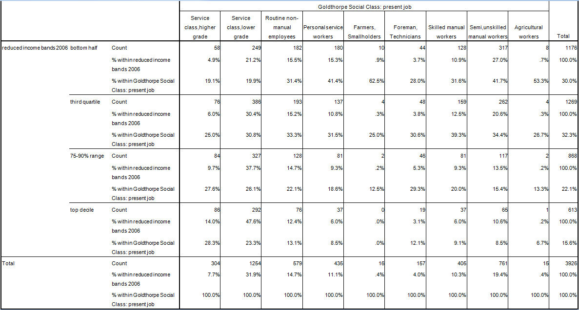
1.6 Evidence from the 2006 wave of the BHPS demonstrates that this assertion is questionable. If we examine individuals who are working and not over the age of 60 for whom a Goldthorpe rank can be assigned, the rank order correlation between household income band and Goldthorpe class rank is just 0.252. The relationship between personal income band and class rank is stronger at 0.352 demonstrating the importance of multiple earners in relation to household income but even so this accounts for just 12% of the variation of even personal income. If we examine all non-retired individuals, Table One shows that even Goldthorpe's Higher Service Class is quite widely distributed through the income distribution. Whilst there is certainly an evident relative concentration towards the upper end of the income distribution, nearly 20% of all employed Higher Service Class members are in the lower half of the household income range. There is a strong relative concentration of Higher Service Class members in the top 5% of households by income but interestingly more than three times as many of those in this elite category come from the lower service class (the largest contributor to the category by far) and more than a third of the category (twice the proportion from the higher service class) come from lower down the Goldthorpe scale.[2]
| Table 1. Income bands 2006 * Goldthorpe Social Class: present job |
|
1.7 For us any specification of class which does not incorporate some sort of direct measure of material resources is fatally incomplete. This is not simply a matter of arguments in class theory, although it seems strange that any work done in a Weberian tradition[3] should not attempt a direct measure of monetary resources. It is also a fundamental problem in relation to what Ragin (1992) calls the problem of casing, that is the crucial decision as to just what is our proper object of interest.
1.8 DiPrete and McManus (2000) identify the problem in clear terms:
'The link between individual occupational mobility and household income mobility has always been somewhat problematic. But the reality of a weakening empirical connection between these two phenomena following a quarter century of rapid change in post-industrial societies underscores the current need for a direct approach that can identify dominant patterns and cross-national variation in the relative importance of labor (sic) market, state, and family mechanisms that affect income'. (2000: 344)
1.9 The proper case for understanding social situation, certainly in terms to market derived command over resources the central core of any Weberian conception of class as opposed to status is the household since in contemporary societies households are the most important units which control and dispose of such resources. This is our casing decision. We must define how household is operationalized but households matter.[4] Understood in this way, mobility is about how individuals and households it is very important to say individuals and households move through time. Class mobility must be, at least in considerable part, about how they move through time in relation to economic resources. The emphasis on the mobility of both individuals and households is necessary because through time individuals move through households just as through time households move through locations in the pattern of resource distribution. So if we are going to explore social mobility in relation to economic resources then we need to do so by recognizing this complex set of mutually interwoven trajectories.
1.10 When class is defined in relation to distribution of economically determined life chances it must be conceptualized in relative terms.[5] Here that will be operationalized in terms of the gross annual cash income[6] location of a household in terms of percentile ranges. This is an incomplete measure taking no account of wealth in any form nor of the expenditure commitments of households, either in terms of household size and age structure the basis on which measures of equivalency are calculated[7] or of acquired assets representing a real income e.g. a 'paid off' owner occupied dwelling. Nonetheless it does measure something of enormous relevance to life chances. We will focus on mobility into or out of the top decile of the household income distribution because that decile stands in a very particular social relation to the rest of the set of households. In particular as, Byrne and Ruane (2008) show, household incomes of the top decile move very rapidly away from the incomes of deciles below them.
1.11 Let us return to the issue of the complex interwoven trajectories of individuals and households. Here we can demonstrate the issues by reference to the logic of the data source which informs the empirical elements in this article, the British Household Panel Survey (BHPS). The BHPS began from a sample of households but households are unstable entities and the only element which can serve as frame across time was the individual. So the constant across time referent in the BHPS is the individual drawn from the set of individuals in the original BHPS panel households or found in any household which has contained an original panel individual at a subsequent wave. Thus the BHPS does not provide us with a panel of households across time but with a panel of individuals together with information about the households containing those individuals. It gives us rich information about both collective household properties and the characteristics of all household members, but the connecting strand is the individual and only individuals possess a unique identification number which is constant across all survey waves.
1.12 A consequence of our approach is that this study belongs in what Savage and Egerton (1997: 647 ) describe as 'the status attainment tradition' in which the emphasis is not on 'aggregate mobility to or from given social classes' but rather on 'the factors which allow individuals [original emphasis] to move up or down the social ladder.
1.13 A fundamental position taken here is that it is not sensible to pursue our understanding of social causality in terms of abstracted variables. Abbott's severe denunciation of this approach bears a lot of repetition.
'The people who called themselves sociologists believed that society looked the way it did because social forces and properties did things to other social forces and properties. Sociologists called these forces and properties 'variables'. Hypothesizing which of these variables affected which others was called 'causal analysis'. what made social science science (original emphasis) was the discovery of these 'causal relationships'' (Abbott 1998: 148-9)
1.14 Goldthorpe argues that what is required always in the first instance in quantitative sociological work is description, that is to say accounts of how things are and how they are related. (Goldthorpe 2000: 152-3) Here we propose the use of exploratory QCA as a means of description. This differs from the usual logic of QCA as developed by Ragin (1987, 2000). Using QCA in this way is, nonetheless, entirely compatible with his insistence that what matter in the social world are not relationships expressed in terms of the causal powers of variables but rather set theoretic relationships.[8] Here we want to go no further than describing set theoretic relationships although we do so in Goldthorpe's spirit of thereby suggesting causal accounts which can be developed on the basis of further investigation. Where we differ from classical uses of QCA is that we go as far as a binary truth table and no further. So we do not proceed in the same way as Cooper (2006) and Cooper and Glaesser (2008) who use the full repertoire of QCA procedures, including the use of fuzzy set approaches, to explore precisely social mobility, albeit social mobility measured in terms which did not include incomes. We do not engage in a reduction in order to establish limited set theoretic configurations associated with an outcome. This is not because we actually have very few fully resolved configurations i.e. configurations in which all the cases have the same value in relation to our binarized outcome pattern,[9] but rather because we are being deliberately exploratory in our approach. We want to see patterns and stop there.
1.15 It would be possible to extend our investigation by looking for additional attributes which would produce a more fully resolved specification of the relationship between configuration and outcome. Byrne (2009) proposes a method for doing this but the most important aspect of his approach is that he looks within particular 'contradictory' configurations rather than trying to add more attributes to the data set as a whole. In other words he engages in a kind of multi-stage comparison based on patterns identified in an original truth table. We do not go that far. Instead we use QCA as a descriptive and exploratory tool.
1.16 The logic of this approach can be demonstrated by comparing what is being done here with the approach adopted in a range of studies e.g. Erikson and Goldthorpe (2010). The starting point for both approaches is a multi-dimensional contingency table. A table is constructed in which all the attributes of cases are arranged across a set of dimensions equal to the number of attributes and cases are located in the cells of that table. Erikson and Goldthorpe construct a log-linear model. That is they specify a model in terms of a set of attributes which is less complete than the saturated model[10] and then compare the pattern of case location across the cells of the multi-dimensional table as generated by this model with the actual distribution of cases. The objective is parsimony explanation in terms of a set of causal variables and interactions among them[11] which does not include all variables and all interactions.
1.17 We instead present a 'combined truth table'. This is a table comprising all the cells in the multi-dimensional contingency table which describe relationships with the outcomes in terms of location across the whole household income range. This is an effective and comprehensible way of presenting an elaborated contingency table. We have 'merged' truth tables so we can see patterns in relation to distribution across household income bands. So our outcome becomes multi rather than bi-nomial. We do not actually see specific interactions between variables.[12] Rather we see descriptions of set theoretic relations which 'embody' all the complex interactions within the causal processes affecting the life trajectories of the complex systems which are individuals through the complex systems which are households. In contrast with the log-linear approach there is no reduction. We see all the patterns in the data. We think this corresponds with what Goldthorpe was seeking when he called for : ' . representations of the data [which] might serve to suggest causal accounts.' (2000: 152) Incomplete configurations can do no more than this. There is always something else going on, in interaction with everything else, for each individual through time.[13] However, we can at least see the patterns, however incomplete, for all our cases, when we work in this way.
1.18 In this context it is interesting to note Jenkins' remark that:
' most descriptions focus on some average experience They do not reveal the diversity of income trajectories, even among individuals with similar characteristics.' (2001: 15)
1.19 We agree but even the sophisticated forms of variable based modelling deployed by Jenkins in relation to his exploration of 'poverty dynamics' do not reveal that diversity. Presentation of a full attribute truthtable does exactly that, especially when as here we present 'composite truth tables'. That is to say we have used the fsQCA software to generate truth tables for outcomes describing the full range of household income categories in 2006 and then brought these together so as to indicate membership of each of the income categories for every configuration. So we are able to see not only the relationship between the configuration of 'causal' elements and a specific location in the household income distribution but rather the relationship of the configuration to the household income distribution as a whole.
What determines individual membership of households by household Income?
2.1 What factors might, in interaction which is a very important notation, have a determinant influence on the interwoven individual and household income trajectories over time? By that expression we mean how individuals' membership of households with particular incomes changes over time and we will measure this by taking the household income of households in which individuals are located at particular time points. These factors are not going to be understand here as independent variables. Instead they are regarded as components of causal sub-systems which are exactly equivalent to Ragin's (2000) specification of configurations. The patterns of causality will be explored by use of Ragin's crisp set Qualitative Comparative Analysis and causality will be understood in set theoretic terms. However, thinking about possible component descriptors of such sets, in Byrne's (2002) terms, traces of them, is appropriate. Normally in QCA this derives from very careful attention to specific cases in a small to medium N set, which often is the whole population of possible cases. Here we will be working with a large N sample of cases drawn from a large population but there are now ample precedents for this approach, f or example Cooper (2006) and Cooper and Glaesser (2008). Even with very large data sets containing thousands of cases we can draw on our general knowledge, derived from both systematic social scientific research and everyday experience of contemporary lives, to identify a set of attribute factors which together in interaction might have an effect on household income at a given time point.2.2 Where people start from in terms of household income category, what qualifications they acquire which might modify their income acquiring capacity, both these factors for all adult household members usually of course each of a couple since couple adult households are absolutely modal in contemporary societies,[14] the number of income recipients, the occupational category of household members, and whether or not those household members are retired, are all potential causal elements. The above set is incomplete. We have no measure of wealth, including in particular of inherited wealth, and wealth is amongst other things a stock which generates incomes. Wealth is particularly important in terms of the life chances of retired households, not least because of the real income generated by owning a dwelling free of payments for it the imputed income which used to be taxed through schedule D in the UK until 1963. The way households have worked, (the active verb is very deliberate), the housing market has had profound implications for marketable wealth.
2.3 The approach taken is to look at household incomes classified in relation to the internal variation in the range of incomes for individuals for whom we have household income for both the years 1992 and 2006.[15] The data set we have created does not describe a set of households. Rather it describes a set of individuals in terms of the both some characteristics of the households of which they are members and some individual characteristics. So we are exploring the relative household income location of individuals over time. We cannot for the reasons explained above explore household trajectories. This is not just a matter of the limitations of the data set. It also reflects the actual reality of the complex double trajectory of individuals through households and households through time. To carry out this exploration we have to create a data set which relates the relative household incomes of individuals at different time points to each other and consider other factors which may enter into our set theoretic relationships. Here we have done this by taking household incomes at time one 1992 and time two 2006. At the individual level we have recorded, from the 2006 data set, for those who are working whether or not they are in the 'combined Goldthorpe service class.[16] We have also noted possession of higher qualifications, whether or not they have managerial responsibilities, their banded age, gender, whether or not they have a partner, and if their partner is employed .
Data limitations
3.1 There are limitations in the BHPS data. There is erosion over time in terms of loss of cases and the BHPS documentation (Lynne 2006) notes that both in terms of initial contact and this process, the data set under-represents households in the bottom 40% of the income distribution. In terms of presentation of aggregate statistical descriptions etc. this issue is usually resolved by weighting but in our view this approach, although the only one available, still has severe limitations because the cases we don't know about are always likely to be different from the cases for which we have information.[17] Because we start with individuals in 1992 of course we do not have information ab initio for all individuals in 2006-6 households, not only because of data erosion but because individuals will have been recruited into the panel at subsequent dates. We started with 5,227 households in 1992 for which we have total household income data. These households contained 9,845 individuals with BHPS unique identifiers. In 2006 there were 14,717 individuals in the data set for which household income data was available but only 5,063 individuals were present at both time points. As with all large data sets there are some missing data and this issue further reduces our actual number of cases available for QCA to 4,873. All income ranges are based on percentiles calculated for those cases for which we have data at both time points but we should note that just 43% of these cases came from the bottom half of the income distribution in 1992 whereas 57% came from the top half.3.2 Ideally we would like to have created a data set which described households in 2006 and had this information for all adult individuals in the households but we could not do this because we lost far too many cases when we attempted to do so. This reflects both data erosion and the impact of new individuals being recruited into the panel over time through common household membership with an original individual member. This means that we can only record the decile of origin of individuals and not the decile of origin of other adult members (usually partners) in their households. Likewise we can only record the educational level and 'combined Goldthorpe service class' of individuals and not of other adult members of their households. We can record if a partner is present and if present is working but our data set is incomplete in terms of the factors which in interaction as configurations are likely to be causal to household income at a time point. We cannot construct a past history for all members of a 2006 household. So we have some relevant 'traces' but not all.
3.3 These issues limit our exploratory / explanatory ability but we have to work with what have and to put it bluntly we have a good deal more here than most studies which deal only with individual trajectories and therefore cannot address the issues raised by DiPrete and McManus (2000) (see above). It is very important to report on data limitations, particularly in relation to erosion in longitudinal studies. This is a general problem and is far too often elided in published work. Gorard's (2008) trenchant critique of Blanden et al.'s influential study (2006) is in considerable part founded around an identification of data limitations and in particular missing data. The great majority of quantitative accounts across time encounter erosion and large survey data outputs are full of 'missing data'. We must as a general practice, identify the limitations of the data we are working with.
Movement across Household Income Deciles between 1992 and 2006
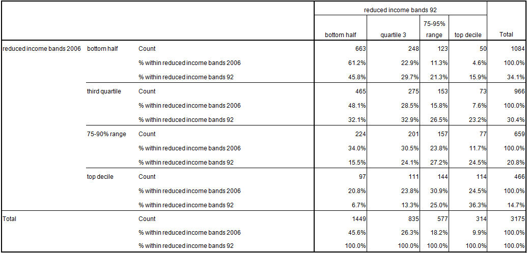
4.1 We start by looking at a simple cross-tabulation for non-retired individuals of the income decile of the household to which they belonged in 1992 against the income decile of their household in 2006[18]. This relationship is very strongly significant and the Spearman's r (these are ordinal variables) is 0.343. The table shows that of those who were in top decile income households in 1992. 36% remained there in 2006 and a further 25% were in the 75-90% household income band at that date. Just 16% of these individuals were in households in the bottom half of the income distribution in 2006. In contrast just 7% of individuals from households in the bottom half of the 1992 income distribution were located in households in the top decile in 2006. There is a good deal of movement evident in this table but the great bulk of it is relatively short range. If we look at the individuals in top decile households in 2006, just under 80% of them came from the top half of the 1992 household income distribution and 55% came from the top quartile. 25% came from the top decile.4.2 What are the patterns associated with this movement, with what Jenkins (2011) calls the spaghetti tangle of trajectories? Looking at configurations enables us to disentangle and see just what is going on.
| Table 2. Percentages of cases within household income band in 2006 by household income band in 1992 for non-retired individuals[19] |
|
4.3 In the remainder of this paper we will focus on the interpretation of QCA generated truth tables generated with individual presence in the top decile of household incomes in 2006 as a particular focus although in Table 3 we show the presence in all income bands in 2006 for each configuration . Here each line in the truth table (configuration) constitutes a specification of the character of a cell in a multi-dimensional cross tabulation with each binary attribute i.e. present or absence of a characteristic, being one dimension in that cross tabulation. In a crisp-set or binary truth table where each 'causal'[20] attribute is either present or absent, then for n attributes there are 2n possible configurations, which are assemblages (a word used quite deliberately here) of possible attributes. So for the thirteen attributes represented in Table 3 there are 8,192 possible configurations. Some of these configurations have no cases present and some have very few. Table 3 contains the 388 (4.7% of all possible configurations) with cases present. Very few are wholly resolved i.e. have either 100% or 0% of the cases for any income band in 2006. That does not worry us. We are interested here in broad patterns and it would be necessary to go further in terms of attribute description to arrive at full determination.[21]
4.4 In all truth tables 1 indicates that the attribute is present. 0 indicates that it is absent. The attributes used are:
- Bottom Half of household income distribution 92.
- Third Quartile of household income distribution 92.
- Range 75-90% of household income distribution 92.
- Top decile household income distribution 92.
- Age Band
- Less than 40
- 41-60
- More than 60
- Gender (0 here indicates Female).
- Has Higher Qualification at least first degree or equivalent.
- Has Partner
- Partner employed
- Present Occupation is Goldthorpe Service Class
- Has Managerial responsibilities
4.5 TABLE 3 is very large but easy to interpret since all that is required is to read across a row (configuration) and see the percentage of cases with that configuration in each 2006 Income Band and the percentage of each 2006 income band coming from cases in that configuration.[22] So the whole available sample is fully described. Here will simply comment on key configurations of interest. Given our focus on access to the top decile we will here comment on configurations which have more than 30% of their cases within that decile. That is to say cases within this configuration have a three times higher presence in the top decile than is the case for cases considered as a whole.
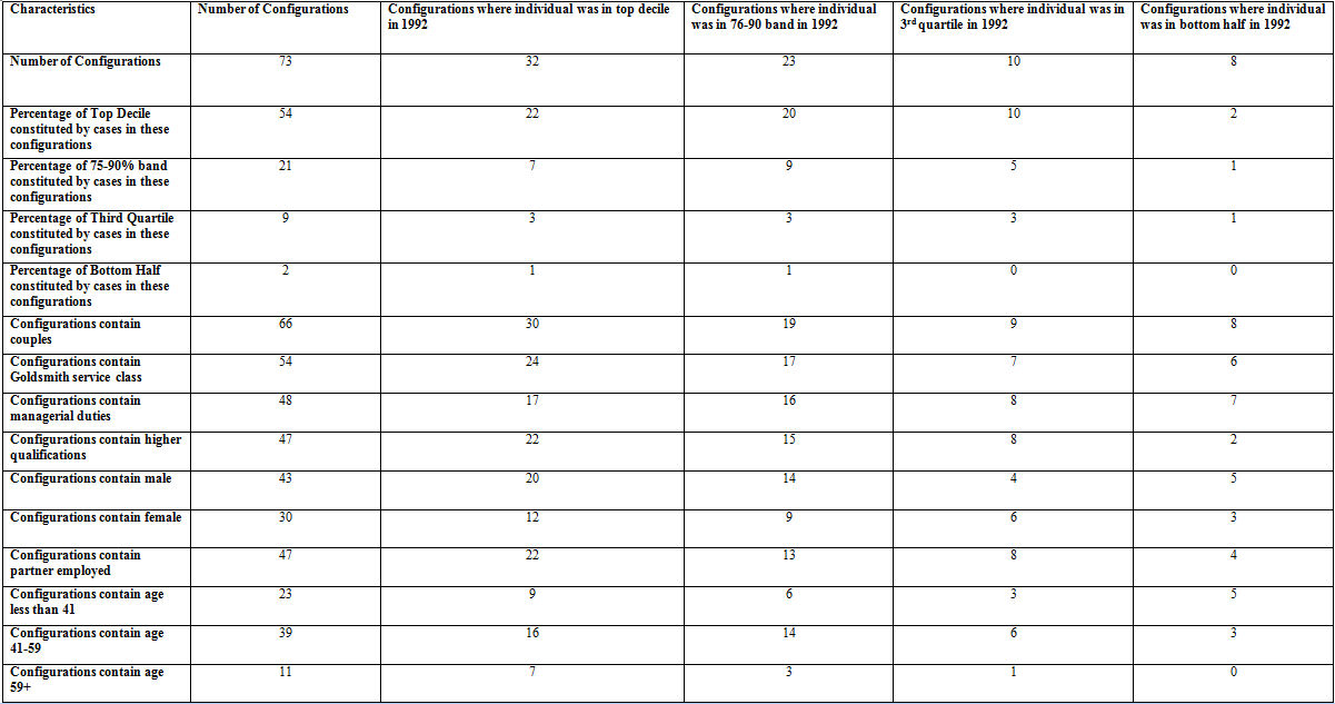
4.6 Table 4 outlines the characteristics of these configurations in aggregate. To determine the character of a configuration read along the line in the data view in SPSS or the EXCEL file. So for example configurations 26 and 27 (with configurations sorted by total number of cases) each contain 40 cases but are:
- 26 men, in couple, partner working, aged 41-59, higher qualification, service class, manager, 92 quartile3, %s in 2006: top 38, 76-90 30, quartile3 28, bottom half 5.
- 27 women, in couple, partner working, aged 41-59, service class, not manager, 92 quartile3, %s in 2006: top 33, 76-90 33, quartile3 20, bottom 13. Configurations 33 (35 cases) and 36 (33 cases) are very similar to the above but have interesting differences:
- 33 men, in couple, partner working, aged 41-59, higher qualification, service class, manager, 76-90 band 92, %s in 2006: top 51, 75-90 31, quartile3 17, bottom half 0.
- 36 women, in couple, higher qualification, manager, 76-90 band 92, %s in 2006: top 55, 76-90 21, quartile3 24, bottom half 0.
4.7 If we take those cases who in 2006 were aged 40 or less, and thus in 1992 were aged 27 or less, then we find some interesting patterns. This group comprises 792 cases spread across 192 configurations. If we sort the configurations in descending order by the proportion of the top decile they comprise, then we find the top three configurations are:
- 34 cases, female, couple, partner employed, higher qualification, service class, not manager, bottom half 92. %s in 2006: top 25, 76-90 32, quartile3 25, bottom half 20.
- 11 cases, female, couple, partner employed, higher qualification, service class, not manager, top decile 92, %s in 2006: top 46, 76-90 18, quartile3 37, bottom half 0.
- 7 cases, female, couple, partner employed, higher qualification, service class, manager, top decile 92, %s in 2006: top 57, 76-90 29, quartile3 14, bottom 0.
4.8 The general indication is that origin in the top decile adds considerable advantage in terms of household income location against those originating in the bottom half of the income distribution although as is inevitable with this considerable partition of the data set it is difficult to establish significance for detailed configurations.[23] In relation to this younger age group it is worth noting that of those in it who were students in 1992, more than 50% are found in households in the top half of the income distribution in 2006, whereas for those who were not this is the case for only 18%. So configuration A above contains women who were in households in the lower half of the income distribution in 1992 but all had obtained higher qualifications and had employed partners. Although this relatively large group included 8 cases in the top decile in 2006, the smaller group C which included those who started in households in the top decile in 1992 included 4 cases in the top decile in 2006. This category had twice the proportionate presence in the 2006 top decile of category C.
Conclusion
5.1 If we think that available economic resources are important for life chances and that the most important unit both possessing and managing such resources is the household, then we must pay attention to household incomes. Income does not describe the whole of household resources but it is important. In societies where the great majority of more affluent non-retired adults work, one of the most important consequences of the feminization of the labour force in post-industrial capitalism, then households are even more important for understanding the nature of social inequality. This is also important in relation to inter-generational transmission of inequality since given the very strong contemporary UK association between being privately educated at the secondary stage and access to elite universities, professions and other elite occupational roles, a relationship which has strengthened in the last twenty years, then high household incomes which can be used to pay school fees, are a positive feedback mechanism enhancing on-going increased inequality.[24]5.2 The actual ways in which individuals move through households and both households and individuals move through the income structure are complex, multiple, and highly varied. Changes in individual income consequent on social mobility and life stage matter, but in terms of household income so do the ways in which households form, dissolve, and reform. DiPrete and McManus (2000) are absolutely right to point out that in contemporary post-industrial societies the link between individual occupation and household income, even between individual income and household income, has become substantially weakened.
5.3 We can attempt to describe complex, multiple and varied movements across time in terms of statistical models. However, such models inevitably 'compress' variation. Moreover, they are very poor at dealing with complex causation. They can only address it, and then only partially, by the insertion of high order interaction terms which is both clumsy and seldom done. The presentation of a full set of real configurations does describe all of what is happening. There may seem to be a data overload but in fact careful reviewing and interpretation of a truth table is not a difficult task. Note the emphasis on interpreting. Patterns do not speak for themselves although they certainly suggest. Table 3 does not give us a conclusive causal account of individuals' movement through household income locations, but it does give us a very extensive and useful exploratory description of such movement.
5.4 The final point to be made here is John Westergaard's repeated. Of course social science should pay attention to how the poor become and stay poor. But it should devote at least as much attention to how the affluent become and stay affluent.
| Table 4. Details of configurations with more than 30% of cases in the top household income decile in2006 |
|
Notes
1There are studies e.g. Buhlmann (2010) which pay attention to the more complex trajectories of actual lives. Longitudinal studies using panels allow for us to explore trajectories across time rather than just in inter-generational terms but it is inter-generational mobility considered in terms of two states which has dominated attention both in the social scientific literature and in recent political debate.2Political discussion has emphasized the obtaining of higher educational qualifications as a means to social mobility, but whilst this may be a helpful attribute (i.e. not absolutely necessary but increasing the probability of higher income) it is by no means sufficient. In 2005 20% of those whose highest educational qualification was at least a first University degree or equivalent were in the bottom half of the household income distribution and for those with any BHPS defined higher qualification the proportion was 27%. Taking account of the impact of retirement by looking only at this relationship for those aged 60 or less, the figures were 18% and 23% respectively.
3This is certainly the dominant frame of reference see Breen 2004 for a discussion in these terms.
4Our operationalization was determined for us, as is invariably the case for studies of this kind which take the form of secondary analysis of available large data sets and there is no other practical way of exploring life trajectories. It is the household as defined in terms of the unit of collection of data by the British Household Panel Survey. That is to say it comprises those people resident at a common address and defining themselves as a discrete household in terms of pooling common resources. This may be a single person or multiple people. This operationalization does not allow us to explore the very important ways in which economic resources are moved around family units defined in extended terms but it is what we have to work with. See Jenkins 2011 for a full discussion of operationalizations in the BHPS.
5The use of relative here is separate from the debate about absolute and relative social mobility for which see Patterson and Iannelli (2007). This has been conducted in relation to 'class' defined in occupational terms. It therefore revolves around the significance attached to changes in occupational structure. Here we deal only with relative incomes across the whole income structure and deciles are deciles at any point in time when incomes are measured.
6We use gross annual cash income because this is what the BHPS measures. However, there is a close relationship between real gross income and post tax income for households when indirect taxes are taken into account. See Byrne and Ruane (2008). In fact the lowest decile of households by income lose the greatest proportion of their income in terms of total tax take but for other deciles the proportion is roughly constant. The use of net income i.e. net of direct taxes, seems to us to be very much mistaken since by doing this studies ignore the very regressive impact of indirect taxes on low income households. The use of relative position also means that we do not need to consider the relationships between incomes and price structures. Income here refers to all cash income received by a household from whatever source. Jenkins (2011) discusses the exact operationalizations of BHPS measures at some length.
7Calculating equivalency is important in studies of poverty but we assert that this is not appropriate when examining very high incomes since the income additions which permit lifestyles and expenditures 'over and above the normal' are not very much affected by household numbers or ages. So for example the purchase of private secondary education is a cost which is influenced by numbers of children of the relevant age but since few households have more than two, this is not a major effect.
8The term set-theoretic is due to Charles Ragin (1987, 2000) and is central to Qualitative Comparative Analysis. Ragin's argument is that causal relationships in the social sciences are generally expressed, and often best understood and explored, not in terms of relationships among abstracted variables but rather in terms of sets of associated attributes which are considered to have causal powers. Theoretical propositions are generally expressed in this way rather than through statements of relations among variables. So set-theoretic techniques, and in particular QCA, are methods which enable the exploration of set relationships themselves.
9We have few configurations with significant numbers of cases in them which reach the rather arbitrary value of 80% concordance which Ragin (2000) suggests we recode as full concordance. This issue relates to our views on deterministic explanation in terms of set theoretical relationships.
10A model in which all possible attribute relationships and interactions are permitted. This simply reproduces the original table.
11Actually interaction terms are very seldom inserted in such models in practice, important though they may be in reality.
12Since we, following Abbott and Ragin, dismiss the causal power of disembodied variables, then this is irrelevant
13And the fallacy of affirming the consequent matters even in relation to completely resolved configurations.
14A major criticism of studies based on longitudinal data sets derived from cohorts is that they do not adequately deal with all the social relational elements which have great significance for life trajectories. Here we at least take account of 'the significant other' although only in a very limited fashion.
15The 1992 wave of the BHPS was the first wave to include useful household income data and at the time of data preparation the 2006 wave was the most recent wave available, although waves up to 2009 have since become available.
16Non workers and workers not in the combined Goldthorpe Service Class are both classified as zero here in the binary attribute.
17Statistical theory spends an enormous amount of time on details of sampling in probabilistic terms but usually neglects this crucial issue of the representative character of the achieved sample.
18Non-retired because retirement transforms household income.
19Household incomes change dramatically on retirement at least as measured in cash terms which do not take account of real incomes from asset possession. Differentiating between non-retired and retired households is conventional. See for example Barnard (2010).
20Of course we establish associations and cannot assert without committing the fallacy of affirming the consequent that these are actually causal, but that is the general problem in relation to causation.
21A somewhat vacuous criticism of QCA is that it is deterministic rather than probabilistic. There is a serious argument to be had about the notion that social cause is inherently probabilistic. Often this arises from a confusion between the necessarily probabilistic status of sample derived statements and reality itself. See Byrne (2002) for a development of this point.
22We have made Table 3 available as both an Excel file and a fully described SPSS file. This means that it can be sorted by any variable. So if you sort it by for example top decile in 1992 in descending order, it will bring all configurations (cases) to the top where the case has that attribute. This makes inspection much easier.
23There is an issue as to whether these differences of proportions are statistically significant. The difference between A and B is not significant for proportion in top decile but the difference between A and C approaches significance. For the whole set of these cases the difference by income band of origin is highly significant but when we try to distinguish in detail we can only say that if women are both managers and originate in the top decile of household incomes, then they approach having a statistically significant advantage over women who otherwise resemble them in terms of a set of positive attributes but are not managers and originate in the bottom half of the household income distribution. If we were able to pool data across a number of years then this might resolve the issue of significance but since the cases are the same year on year would these constitute independent samples appropriate for pooling?
24One surprising omission from the BHPS data base is information about the type of school attended by children in households so we cannot map this relationship but it is evident logically and on the basis of other available evidence.
References
ABBOTT, A. (1998) 'The Causal Devolution' Sociological Methods and Research 27 (2) 148-181. [doi:://dx.doi.org/10.1177/0049124198027002002]ABBOTT, A. (1988) 'Transcending General Linear Reality' Sociological Theory 6 169-186. [doi:://dx.doi.org/10.2307/202114]
BARNARD, A. (2010) The Effects of Taxes and Benefits on Household Income, 2008/09, Office for National Statistics, 2010 (http://www.statistics.gov.uk/CCI/article.asp?ID=2440).
BLANDEN, J., Gregg, P. and Machin, S. (2005) Intergenerational mobility in Europe and North America: Report for the Sutton Trust, London: Centre for Economic Performance
BREEN, R. (ed.) (2004) Social Mobility in Europe Oxford: Oxford University Press.
BUHLMANN, F. (2010) 'Routes into the British Service Class' Sociology 44 2 195-21.
BYRNE, D.S. (2002) Interpreting Quantitative Data London: Sage.
BYRNE, D.S. (2009) 'Using Cluster Analysis, Qualitative Comparative Analysis, and NVIVO in Relation to the Establishment of Causal Configurations with Pre-existing Large-N Datasets: Machining Hermeneutics' in Byrne, D.S. and Ragin. C. (eds) The Sage Handbook of Case Based Methods London: Sage 260-268.
BYRNE, D. and Ruane, S. (2008) The UK Tax Burden: Can Labour be called the party of fairness? Compass at: <http://clients.squareeye.net/uploads/compass/documents/Fairness%20Thinkpiece%2040%20REVISED_%20(2).pdf>.
COOPER, B. (2006) 'Applying Ragin's Crisp and Fuzzy Set QCA to Large Datasets: Social Class and Educational Achievement in the National Child Development Study' Sociological Research Online 10 2.
COOPER, B. and Glaesser, J. (2008) 'How has Educational Expansion Changed the Necessary and Sufficient Conditions for Achieving Professional, Managerial and Technical Class Positions in Britain? A Configurational Analysis' Sociological Research Online 13 3. [doi:://dx.doi.org/10.5153/sro.1703]
DIPRETE, T.A. and McManus, P.A. (2000) 'Family Change, Employment Transitions, and the Welfare State: Household Income Dynamics in the United States and Germany' American Sociological Review 2000 65 343-370. [doi:://dx.doi.org/10.2307/2657461]
ERIKSON, R., and Goldthorpe, J. (2010) 'Has social mobility decreased? Reconciling divergent findings on income and class mobility' British Journal of Sociology 61 2 211-230.
GERSHUNY, Jonathan (January 2002a) 'A new measure of social position: social mobility and human capital in Britain', Working Papers of the Institute for Social and Economic Research, paper 2002-2. Colchester: University of Essex.
GOLDTHORPE, J. (2000) On Sociology Oxford: Oxford University Press.
GOLDTHORPE, J. (2001) 'Causation, Statistics and Sociology' European Sociological Review 17 1 1-20.
GORARD, S. (2008) 'A re?consideration of rates of 'social mobility' in Britain: or why research impact is not always a good thing' British Journal of Sociology of Education 29 3 317-324
JENKINS, S.P. (2011) Changing Fortunes Oxford: Oxford University Press. [doi:://dx.doi.org/10.1093/acprof:oso/9780199226436.001.0001]
LEISERING, L. and Walker, R. (1998) 'New Realities: the dynamics of modernity' in Leisering and Walker eds The Dynamics of Modern Society Bristol: Policy Press 4-5.
LYNNE, P. (2006) Quality Profile: British Household Panel Survey Version 2.0: Waves 1 to 13: 1991-2003 Institute for Social and Economic Research University of Essex.
PAKULSKI, J. and Waters, M. (1996) The Death of Class London: Sage.
PATTERSON, L. and Iannelli, C. 'Patterns of Absolute and Relative Social Mobility: a Comparative Study of England, Wales and Scotland' Sociological Research Online 12 6 15.
RAGIN, C.C. (1987) The Comparative Method: Moving beyond Qualitative and Quantitative Strategies Berkeley CA: University of California Press.
RAGIN, C. (1992) 'Casing and the process of social inquiry' in C. Ragin and H. Becker (eds) What is a Case? Cambridge: Cambridge University Press 217-226.
RAGIN, C.C. (1994) Constructing Social Research Thousand Oaks CA: Pine Forge Press.
RAGIN, C. (2000) Fuzzy Set Social Science Chicago: University of Chicago Press.
SAVAGE, M. and Edgerton, M. (1997) 'Social Mobility, Individual Ability and the Inheritance of Class Inequality' Sociology 31 4 645-672.