Damaging the Case for Improving Social Science Methodology Through Misrepresentation: Re-Asserting Confidence in Hypothesis Testing as a Valid Scientific Process

Background

1.1 This paper is a response to Gorard's article, 'Damaging real lives through obstinacy: re-emphasising why significance testing is wrong' in Sociological Research Online 21(1). For many years Gorard has criticised the way hypothesis tests are used in social science, but recently he has gone much further and argued that the logical basis for hypothesis testing is flawed: that hypothesis testing does not work, even when used properly. We have sympathy with the view that hypothesis testing is often carried out in social science contexts when it should not be, and that outcomes are often described in inappropriate terms, but this does not mean the theory of hypothesis testing, or its use, is flawed per se. There needs to be evidence to support such a contention. Gorard claims that: 'Anyone knowing the problems, as described over one hundred years, who continues to teach, use or publish significance tests is acting unethically, and knowingly risking the damage that ensues.' This is a very strong statement which impugns the integrity, not just the competence, of a large number of highly respected academics.

1.2 We argue that the evidence he puts forward in this paper does not stand up to scrutiny: that the paper misrepresents what hypothesis tests claim to do, and uses a sample size which is far too small to discriminate properly a 10% difference in means in a simulation he constructs. He then claims that this simulates emotive contexts in which a 10% difference would be important to detect, implicitly misrepresenting the simulation as a reasonable model of those contexts.

1.3 We will not address all of the shortcomings we see in Gorard's paper, and the absence of criticism of particular aspects should not be taken to infer that we agree with what he has written. We feel it is particularly important that the focus be kept tightly on what Gorard claims for his paper – that it presents a series of demonstrations that show significance tests do not work in practice. As such, the following paragraphs work through a number of sections of Gorard's paper as a way of illustrating our argument.

Introduction

2.1 Gorard (2016) provides a one-sided literature review citing articles that are critical of hypothesis tests, but in White & Gorard (forthcoming) he goes further and claims that Authorities now generally agree that ISTs (inferential statistical tests) do not work as intended. We believe that this unsubstantiated assertion is not true – indeed if it were true, it would be difficult to imagine that their use would not have disappeared. As an example of how seriously this claim is flawed we refer readers to The American Statistical Association statement on p values, published on 7 March 2016 which makes the following 6 points:

1. p-values can indicate how incompatible the data are with a specified statistical model.
2. p-values do not measure the probability that the studied hypothesis is true, or the probability that the data were produced by random chance alone.
3. Scientific conclusions and business or policy decisions should not be based only on whether a p-value passes a specific threshold.
4. Proper inference requires full reporting and transparency.
5. A p-value, or statistical significance, does not measure the size of an effect or the importance of a result.
6. By itself, a p-value does not provide a good measure of evidence regarding a model or hypothesis.

2.2 The news release can be found here: https://www.amstat.org/newsroom/pressreleases/P-ValueStatement.pdf and the full paper here: http://amstat.tandfonline.com/doi/abs/10.1080/00031305.2016.1154108.

2.3 This statement clearly takes the view that p values are misused, and are not sufficient evidence on their own, but does not make any criticism of the underlying logic of significance tests – there is nothing in this statement which could be taken to support the assertion that ISTs do not work as intended.

2.4 While this statement was published just after Gorard's article appeared and he could therefore not cite it, articles like Cox and Mayo (2010) authored by one of the UK's foremost statisticians, Sir David Cox, FRS and Professor Deborah Mayo, who holds a visiting appointment at the Center for the Philosophy of Natural and Social Science of the London School of Economics, are available and clearly do not support the contention that statistical testing does not work as intended. We will start by setting out the logic of hypothesis testing, and then attempt to show what is wrong with Gorard's reasoning in his paper. One important complication in doing that, is that Gorard's use of the language of hypothesis testing in the paper is inappropriate in many places: there are inaccurate statements as to what the protocol says. This suggests a misinterpretation of the technique he claims in this paper to show is fundamentally flawed in its theory.

The logical basis of hypothesis testing:

3.1 Statistics is about making sense of incomplete information, and decision making in the face of uncertainty – the source of which may be the incomplete information or randomness associated with events yet to happen. It is important to distinguish between cases where:

• a sensible decision has been taken, but once hindsight is available it is apparent that a different decision would have given a better outcome
• the decision was not the most sensible, given the available information.

3.2 An obvious case is the payment of insurance premiums – if you do not make a claim against the policy then you would be financially better off if you had not paid the premium, but that does not mean that the decision to take out the insurance was wrong: the litmus test is whether you would make the same decision again in the same situation.

3.3 You need to bear this in mind when dealing with hypothesis tests – you are weighing up a situation where incomplete information is all that is available, and needing to make a decision as to what to do in the light of the evidence which is available. Another key aspect of statistics which is central to understanding hypothesis testing and making sensible decisions is to know something about the quality of the information you have: any reporting of outcomes of tests should be couched in terms which remind the reader that this is a judgement based on the available evidence – not a pronouncement of fact or absolute truth. One of the strengths of hypothesis tests is that the power function of the test, taken alongside the p value, gives a very good assessment of the risks associated with any decision – including telling you when you simply do not have enough data on which to make a decision with any degree of serenity.

3.4 There are a multitude of different hypothesis tests in common use. We will provide a detailed explanation of the logic in the context of, arguably, the simplest case – a 2-tailed test for the mean in a context where the population is known to be Normal, and the variance is known, and we will then provide an explanation of the logic underpinning the test Gorard uses in section 4 of his paper – testing a difference between two samples drawn from uniform distributions.

Testing for the mean of the Normal distribution

3.5 A null hypothesis test (NHT) requires both a null and an alternative hypothesis to be stated before any analysis is done (indeed, it should really be done before data is even collected – which would ensure that observations cannot influence the choice of hypotheses). The null hypothesis (^H₀) must provide a sampling distribution for the statistic of interest (in this case the mean) and the alternative hypothesis (^H₁) must identify what will constitute the most unusual outcomes if the null hypothesis is true.

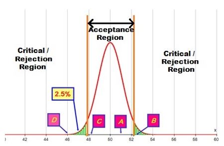
3.6 Let us consider the case where the population is known to be Normal and have a standard deviation of 5 and we wish to test ^H₀: µ = 50. (where µ is the population mean) against ^H₁:µ ≠ 50. If we do not have any reason (before looking at any observational data) to expect an increase or decrease in the mean the default is to test for a difference – in which case the 'most unusual outcomes' will be equally split at the top (values well above 50) and bottom (values well below 50) –and for a 5% significance level this will be the top and bottom 2.5% of the sampling distribution. For our test we are going use a random sample of 20 observations:

3.7 The green shaded regions at the bottom (below 47.81) and at the top (from 52.19 up) each contain 2.5% of the sampling distribution for the mean of a sample of size 20 from this population. These two regions together are known as the critical region or rejection region for the test – if the observed sample mean lies in the critical region then the conclusion of the test would be to reject ^H₀ and say that there is evidence at the 5% level of significance to suggest that the mean is not 50. So sample means at B (52.5) and D (46) would reject the null hypothesis but sample means at A (51) and C (48) would not reject it and you would say that there is not sufficient evidence at the 5% level to suggest that the mean of the population is not 50. The region in the middle is known as the acceptance region – for obvious reasons.

Figure 1. The acceptance and critical / rejection regions for a Normal test of the mean.

3.8 Some readers may not be familiar with this approach to hypothesis testing, and we will show the relationship with p values shortly, but the reason for considering this approach first is that it offers a really strong visual understanding of what is going on in a test, particularly when we consider how effective a test is in picking up any shift in mean which the researcher deems is important.

3.9 We can immediately say that the p values at B and D will be less than 5% (because they lie in the critical region), and those at A and C are greater than 5%, but looking at their positions we could informally deduce rather more – and this can help to build confidence in our understanding of what is happening with p values. D will have a smaller p value than B because it is further along the tail; C will have a p value which is more than 5%, but not a lot more as 48 is only just above the boundary of the critical value; A will have a p value which is much bigger than 5% because it is nowhere near the boundary of the critical region.

3.10 The exact p values are D (0.003%); B (2.5%); C (7.4%) and A (37.1%). This may give some insight into the behavior of p values when researchers try to replicate published studies – see Cumming 2012: 135-138 for a fuller explanation of this characteristic – what he calls the dance of the p values. The p value depends on just where the test statistic falls – this is why the p value on its own is really not enough evidence of the suitability (or otherwise) of a model (ASA 2016).

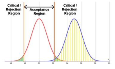
3.11 In the example above, an effect size of 1 would occur when the true population mean is 45 or 55 (which is a 10% shift in the mean). How good would this test be at identifying such a shift in the mean? The diagram below shows what the sampling distribution would be if the mean was actually 55 (in blue) and the yellow shading shows what part of that distribution lies in the critical region – 99.4%, so this test with a sample size of 20 would actually be very good at identifying a shift in the mean as large as 5 – or an effect size of 1. In the language of hypothesis testing, the power of the test at 55 is 99.4%, i.e. you can expect to detect such a difference 99.4% of the time. Visually, it is easy to see that the two sampling distributions are distinctively different, which is why the power is so high. However, an effect size of 1 is a pretty big shift – in social sciences an intervention with an effect size of 1 is rare.

Figure 2. The power of the test for a 10% shift in mean of the distribution in Figure 1.

3.12 The smaller the effect size you feel it is worthwhile for your test to be able to detect (i.e. return an observed value in the critical region of the test, and hence a significant p value) the larger the sample size will need to be. What criteria should be used for 'commonly return a significant p value'? Gorard 2013 has a section on sample size (see pages 85-87) that includes Lehr's approximation, which gives an easy method of calculation if you are not happy with the mathematics involved in an exact calculation. It is based on a significance level of 5% and a power of 80% - it says that the minimum sample size needed for 80% power is (approximately) 16 divided by the square of the effect size (which is the difference in means divided by the standard deviation). In the case above the minimum sample size to meet these criteria would be 16. If the sample size was only 16, both the distributions above would be centred in the same places (as they are currently) but would be more spread out (and less tall in the middle so the total area would stay the same). So the purple section of the critical region (using the red distribution) would move to the right, and also the blue distribution would be more spread out – both changes having an effect in the same direction – reducing the power of the test (from 99.4% to 80%). This is why the size of the sample used in a test is so important – the power is very sensitive to the sample size.

3.13 Let us now consider the example Gorard uses in section 4 of his paper – using a sample size of 100 to test for a difference in means of 10% in a population which is uniformly distributed on the interval (0,1). The mean of that population is 0.5, and the standard deviation is , and a 10% shift in mean will go to 0.45 or 0.55. This has an effect size of 0.173

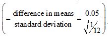
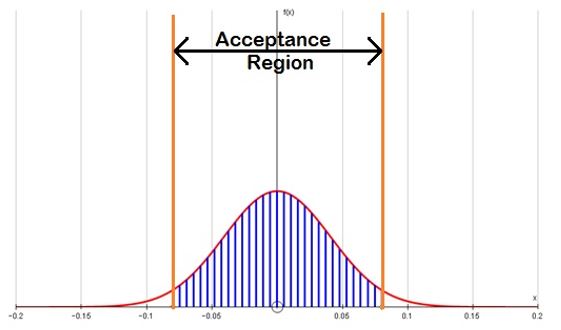
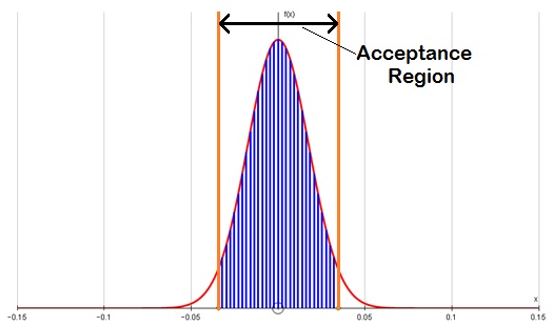
3.14 The diagram below shows the sampling distribution for under ^H₀ (no difference) –the shaded area between ±0.08 shows the acceptance region of the test – any observed difference in means from samples of size 100 lying in this region will not give a significant p value. Note is the sample mean of one set of data and is the sample mean of the other set of data – both with 100 cases.

Figure 3. The acceptance region for a difference in means between two samples of size 100 drawn from a U(0,1) distribution.

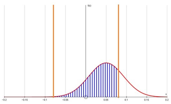
3.15 The diagram below (Figure 4) shows the sampling distribution for the difference in means when the second sample is drawn from a population in which the mean is actually 10% higher (0.55 instead of 0.5) –in this case the distribution also is more spread out than that for the null hypothesis (above).

3.16 The shaded area below shows that with only 100 cases in each sample a very high proportion (76%) of samples drawn with only a 10% difference in means will lie in the acceptance region for the test – because the test is using far too small a sample to discriminate effectively.

Figure 4. The power of the test for a 10% difference in means between two samples of size 100 drawn from a U(0,1) distribution.

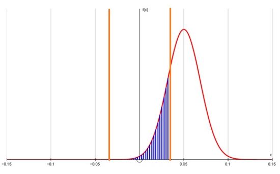
3.17 If you wanted to produce significant differences on 80% of occasions in which a 10% difference in means was actually present then you would need to have a sample with 540 cases in each group (we show the derivation of this sample size later in the paper). The two diagrams below show the sampling distributions which correspond to the two distributions above.

Figure 5. The acceptance region for a difference in means between two samples of size 540 drawn from a U(0,1) distribution.

Figure 4. The power of the test for a 10% difference in means between two samples of size 540 drawn from a U(0,1) distribution.

3.18 Now only 20% of the observed differences in mean will fall into the acceptance region of the test. It should be obvious from this that a random sample of 200 people (100 per group) would predominantly come to the conclusion that there was not sufficient evidence of a difference in means – purely because the sample size used is known to be far too small to discriminate this size of shift for a uniform distribution. Note to readers – figures 3 - 6 above have more white space than you will be used to seeing in most graphs – this is because they are all constrained to have the same x and y scales in order that you can accurately see the comparisons to be made.

Critique of Gorard's paper

Most important issue – does the 'practical demonstration' in section 4 show that hypothesis tests do not work as intended – as Gorard claims?

4.1 The above section shows that the sample size used in section 4 of Gorard's paper is far too small to reliably identify a 10% shift in the mean of a uniform distribution. Gorard certainly should be aware of this as he devotes a section (Gorard 2013: 85-87) in a recently published textbook to explaining the need to compute the minimum sample size which will provide significant outcomes to the test with any probability (less than 1) that you choose to specify, and cites Lehr's approximation for a 5% significance test and an 80% likelihood of getting a significant outcome. Using that approximation in this case gives the following:

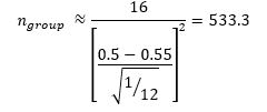4.2 The exact group size needed for a power of 80% can be calculated to be 540 (the second sample size used in considering the logic of the test in the previous section). If he had used a sample size of 100, thinking that that is large, then he might be criticised as simply naive: after all, in the first example we quoted above, a sample size of only 20 gave a power of 99.4% for a difference we wanted to be able to pick up, which was also a 10% shift in the mean! However, as he has had a textbook recently published (Gorard 2013) which addresses the issue of sample size explicitly, including discussing the important role of the variability of the population, then he is obviously not naive.

4.3 Thus we would question the use of a sample size which is far too small, whilst making no reference to the sample size needed resulting in a claim that the observed low rate of significant outcomes is evidence that significance testing does not work as intended.

4.4 If Gorard's simulation using 100 cases had been the correct sample size to give the 80% power he uses in his textbook but only generated 12% of significant outcomes, then he would be correct in claiming that he had demonstrated that significance tests do not work as intended, and indeed this would have been a really important result! However, it is not the correct sample size to give 80% power, and when the correct sample size is used, the simulation does return around 80%, and when 100 cases are used the simulation does return the proportion of significant outcomes that the logic of hypothesis testing predicts it will (which is neither 80% as is the common target, nor 12% as Gorard obtains - see below)..

4.5 We find it disturbing that Gorard has arrived at the conclusion that somehow this 'practical demonstration' shows that hypothesis tests do not work as intended. It categorically does nothing of the sort: the arguments put forward in relation to what the simulation shows are unsupported and we believe misleading.

4.6 Our simulations, with 50, 100 and 540 cases can be downloaded from https://community.dur.ac.uk/j.r.nicholson/ for readers who would like to run them or explore them for themselves, along with a fuller treatment of the mathematics behind Lehr's approximation, the exact calculation of minimum sample size, and what the exact test should be in each case.

Does Gorard misreport the sample size used in his first 'demonstration'?

4.7 We are unable to replicate the results of Gorard's experiment with 100 cases: we note that he reports getting 1217 out of 10,000 simulated samples - which he erroneously refers to as 5.5% before later in the paragraph referring correctly to 'approximately 12%'. The actual power of the exact test is 24%, and Excel consistently returns a slightly smaller proportion of significant t test outcomes, assuming equal variances – typically in the low 20%s – but we have not seen anything approaching 12% after running the simulation many times.

4.8 However, when we run a simulation with 50 cases in each group (a total of 100 cases) we do obtain around 12% significant outcomes in Excel's t test. The text is clear about how the simulation was to be structured (in see section 4.4) –with 100 cases in each group and a total of 200.

4.9 Gorard's paper says that the simulations 'can be replicated easily by all readers'. We think we have replicated the simulation as it is described, but we are unable to replicate Gorard's results. We have made our simulations available online (see above) and invite Gorard to identify what is wrong with them if we have made an error. We also invite him to revisit the simulation file he used and see if it does in fact use a sample size of 100 – if so, he should make it publicly available in the interests of transparency, but if it does use a sample size of 50 this should be acknowledged.

4.10 The misreporting of the sample size used in an experiment by a factor of 2 would be a very serious error in any published paper. It is important that it is cleared up once and for all. The steps above would allow this to be done very quickly. However, this is a procedural error and should not distract from the greater methodological error which lies at the heart of this analysis.

Other issues with section 4 of Gorard's paper

4.11 In section 4.3 Gorard says that 10% is a substantial difference – and tries to use his simulation of the uniform distribution to say that 'large groups' of people with a 10% difference must be detectable – citing emotive examples such as gender bias in earnings, and the difference in death rates if cancer diagnosis took longer for poorer people, as well as heights. We have a couple of problems with this:

• Gorard 2013: 85 – 87 explicitly deals with the influence of the standard deviation of the underlying population on how easy, or otherwise, it will be to pick up any specified difference in means – so the statement (see section 4.3) stating that a 10% difference in means is always a substantial difference appears to us to be both misguided and inappropriate.
• The notion that a uniform distribution is an appropriate model for the population in any of these contexts is mistaken: the uniform distribution has a much larger standard deviation (relative to the range) than most distributions – which typically tail off in at least one direction. The distribution of male adult heights in the UK can be modelled reasonably by a Normal distribution with mean 178 cm and standard deviation 10 cm. A 10% difference in height in such a situation between two groups would be a very large effect size indeed (1.78) and you would expect to be able to identify this is in even relatively small groups where the 10% difference in the uniform distribution has a tiny effect size (0.173) and you need a huge amount of data to identify this – a factor of more than 100 times as large a sample size. To use a 'model' in which the effect size is 10 times greater than the contexts you purport to be modelling and just be talking about the difference in means being 10% in both cases is an oversimplification which misrepresents the underlying data, leading to conclusions which do not withstand closer inspection.

4.12 Also, the wording in these examples suggest that a one-tailed test is what should be used – there is an implication as to the direction any deviation from the null hypothesis of equal means would be in (males earn more; poorer people have higher death rates, males are taller). Gorard fails to state explicitly what the alternative hypothesis is in his article, but uses a 2-tailed test.

4.13 In section 4.4 Gorard says 'It would be no use pointing out that the men in the sample earned around 10% more than the women. The t-test advocate would say 'ah but it is not significant.' Well, no, in fact they would not(!) because a 10% difference in sample means lies in the critical region (the cutoff even on a 2-tailed test is actually 8% - see Figure 1). The following sentence starts 'This is patent nonsense' which we feel is ironically apt. This is gross misrepresentation – the statement about what the t test advocate would say is patently untrue. To repeat, a 10% difference in sample means would be a significant outcome.

4.14 It is also worth noting in passing that he conflates what the population difference is (which in real-life is unknown) with the observed outcome – with a sample size known to be grossly inadequate for the distribution under consideration, the observed outcome will not always be what the population difference is.

4.15 Section 4.5 of the paper in question incorrectly represents what significance testing does. The null hypothesis provides a sampling distribution which can be used to identify the 'most unusual events' if the alternative hypothesis is true. It does not make any assumption that the null hypothesis is actually true. To say that 'The computation of the p-values is now based on a flawed assumption, and so the computed p-values will be wrong in real-life examples' is to display a deep misunderstanding of the logic of significance testing.

A technical note

4.16 The way Gorard has set up his simulation is, simply, wrong and is a misapplication of statistical theory.

• Gorard uses a Uniform distribution as the underlying population for his simulation and uses a t test for the differences between groups. A t test is only applicable when you have to estimate the standard deviation of the underlying population(s), which are well known in this case – otherwise there is always a corresponding Normal test which should be used when the variance is known.
• We believe he has also assumed equal variances in his test, although the variances are known to be substantially different – one is 21% larger than the other.
• He uses a completely inappropriate model for the population distribution if he wants to apply the results of the simulation to any social science context.

Issues with section 3 of Gorard's paper

5.1 It is not the first time that Gorard has failed to articulate the hypotheses in an article. Gorard 2014: 6 states:

To imagine otherwise, would be equivalent to deciding that rolling a three followed by a four with a die showed that the die was biased (since the probability of that result is only 1/36, which is much less than five per cent, of course).

5.2 This is an example of what we referred to earlier – a misapplication of the hypothesis testing protocol – which requires a clear statement of both null and alternative hypotheses before going anywhere near the data. What possible alternative hypothesis would identify a three followed by a four as being an extremely unlikely event under the null hypothesis of a fair die? Nicholson 2015 articulates the criticism of this example more fully.

5.3 In section 3.7 Gorard states:

However, the biggest problem with significance tests is that their logic is fundamentally flawed. They just do not work as proposed, because the probabilities they calculate are not the probabilities that any analyst wants. Significance tests calculate the probability of getting a result as or more extreme than the one that has been observed, assuming that the nil-null hypothesis is true. What analysts want is the probability of the nil-null hypothesis being true, given the result obtained. These two are completely different. Yet when rejecting the nil- null hypothesis on the basis of a p-value the analyst is using the first probability as though it were the second.

5.4 The ASA statement on p values makes it plain that this is not what hypothesis test protocols are doing when the null hypothesis is rejected on the basis of a p value (Wasserstein & Lazar 2016). ASA 2016 is the press release relating to this full paper, and it summarises succinctly many of the issues we have with the way Gorard portrays the protocols of significance testing.

5.5 In section 3.8 Gorard says that significance test advocates claim that drawing 7 red and 3 blue balls from a bag containing a total of 100 balls which are blue and red (in unspecified proportions) can tell us what the colours are of those left. This is, in our view, a gross misrepresentation: I can do a test which will identify the likelihood of getting a 7:3 split, or more one-sided, if the bag had half red, half blue (the p value under the null hypothesis of equal numbers) and I could calculate the power function showing the probability of getting that set of outcomes for any red / blue split of the 100 balls in the bag – but nothing in hypothesis test protocols claim that I can actually tell from this what colours are left. I have some information that I can use to inform any course of action – fully aware that I have incomplete information. Again, ASA 2016 makes it abundantly clear that significance test protocols do not make any such claim.

5.6 Hypothesis testing does not make an assumption of what is in the bag – the p value is based on where the observed outcomes lie in the sampling distribution under the null hypothesis, and one reason for showing the critical region approach for hypothesis testing is to emphasise that significance testing is not done post hoc if it is done properly. Once the hypotheses are specified, which Gorard repeatedly fails to do, the critical region is well defined and the p value could be calculated for any possible observed outcome of the experiment – remember in the introduction to the logic we showed what the p values were for 4 different possible observed sample means. The probabilities of seeing at least as extreme an outcome as a 7:3 split from a bag with 80 red, 20 blue or 20 red, 80 blue balls are actually the power of the test for those two specific cases. Certainly the p values will be the same whether the bag actually contains 20, 50 or 80 red balls – because of what the p value is defined to be.

5.7 We believe that Gorard has misrepresented what hypothesis tests claim to do (as in the above quote from this paper). This might be due to a misinterpretation of the statistical reasoning behind hypothesis testing or perhaps that he feels that they are so often misused that he is justified in claiming that the logic is flawed, even if they are used properly. If he feels that it is the case that the logic is flawed in particular cases where researchers have meticulously followed the protocols, we would request that fully documented examples are provided of where this has been published, and identify the flawed logic – we believe that every example he has cited does not follow hypothesis testing protocol and that is the problem, rather than demonstrating any flaw in the logical basis.

Issues with section 5 of Gorard's paper

6.1 We believe that this entire section is completely redundant as it is claiming to show that something, which has no part of the significance testing protocols, leads to serious mistakes. Gorard claims in section 5.1 that the demonstration 'shows how inverting the probabilities in a significance test, as must be done to 'reject' the nil-null hypothesis, leads to serious mistakes.' However, ASA 2016 makes it abundantly clear that this inversion of conditional probabilities has no place in the protocols of significance testing.

Conclusion

7.1 We believe that there are serious flaws in this article (Gorard 2016) and also in Gorard 2014 where he claims to show that hypothesis testing does not work. We believe that there are many and serious issues about the way hypothesis tests are misused – that many researchers use them in inappropriate situations and conclusions are often inappropriately stated. However, we argue that that the theory itself is not flawed.

7.2 Gorard's paper purports to present 'a series of demonstrations' that show that significance tests do not work. He claims 'anyone knowing the problems, as described over one hundred years, who continues to teach, use or publish significance tests is acting unethically, and knowingly risking the damage that ensues.' This is a very strong statement which impugns the integrity, not just the competence, of a large number of highly respected academics.

7.3 The first demonstration is, we believe, much worse than irrelevant: he uses a sample size which is easily shown to be completely inadequate to distinguish the tiny effect size he wants to pick up - and then says that significance tests don't work because the difference is not commonly picked up. In fact it is picked up as often as the theory predicts it will be. We invite the reader to draw their own conclusion on the ethics of the use or suppression of hypothesis testing.

7.4 We believe that the second demonstration is completely irrelevant as hypothesis testing does not make the claim he says his demonstration shows is untenable: that the direction of a conditional probability can not be reversed is well known, and is much better illustrated by the counter examples he quotes than this exhaustive analysis of all possible combinations. The key fact is that section 5 is a straw man argument because significance testing does not claim that the direction of a conditional probability can be reversed.

7.5 We agree wholeheartedly that testing is often abused within educational research, but we believe the problem is that testing is used in contexts it should not be, and that the outcomes are reported incorrectly - often in addition to an inappropriate context. We think there is a strong case for the proposition that they should not be viewed as the default technique in educational research, and arguably that they should only be used in circumstances where it can be demonstrated that they will be correctly used. However, we believe that there are important improvements with much wider use of proper randomized controlled trials (RCTs). We fear that the demonization of sincere and ethical researchers, who are aware of the intricacies and caveats of these techniques, by an influential figure like Gorard, who has misrepresented the protocols, will hinder researchers and restrict development in research-informed decision-making.

7.6 We fear that the case for improving the use of hypothesis testing will be fundamentally damaged by articles like this which make unwarranted claims that the theory itself is flawed.

References